In Depth Report
A course project website for EECS 349 Machine Learning at Northwestern University
And an artificial intelligent system caring for your health, completely free of charge :)
A course project website for EECS 349 Machine Learning at Northwestern University
And an artificial intelligent system caring for your health, completely free of charge :)
JianXu2020@u.northwestern.edu
RongqiDing2020@u.northwestern.edu
The health and medical care industry is an industry of great importance and intricacy because it is related to everyone. What we’re looking forward to establish is a tool which takes patients’ symptoms (typed in words) as inputs and gives basic diagnose as outputs. A tool like this can be of great use. Patients can use it to get an idea of the potential explanation to their health problems and how severe it is. Doctors and hospitals can use it to assign patients to the most suitable department and reduce the amount of human labor involved.
We used a medical transcription dataset from Kaggle: medical transcriptions. This data set contains around 5000 samples, covering 40 medical specialties. From the various attributes, we made use of “description” and “medical specialty”. The former one is a sentence describing the symptoms the patient is having. The latter one is the professional area or department the patient’s doctor belong to. We split the whole data set in training set and test set with the ration of 7:3. For comparison purpose, the two sets were fixed throughout the process.
Our work can be broken down into three major subtasks: “Word Vectorization”, “Feature Extraction” and “Classification”. The raw input are first preprocessed into vectors using the “bag of words” idea, and then corresponding features (or key words) are extracted separately for every medical specialty (for reference simplicity, referred as ‘class’ in the following report). In the classification process, output value are assigned by the class whose features are what the test sample is closest to. A weighted distance calculation is used in this process.
Our preprocessing procedure contains the following steps. (a) Punctuation: “-” is replaced with “ ” to break down the words before all the punctuations are removed. (b) Regularization: All the letters are regularized to lowercase. (c) Stop Words: Stop words are removed from the sentence. (d) Tokenization: Up to this point, the input is still in “string” form. By tokenizing it, the string is separated into individual words and make up a “list” of word tokens. (e) Lemmatization: To further generalize the applicability of this system, lemmatization is introduced. Words from the same family but with different affixes are grouped into one. For example, “allergies” is swapped for “allergy”. (f) Vectorization: After all the samples are tokenized, a vector marking the number of appearance of all the non-repeat input tokens can be created for every description (Bag of words). After all these steps, the preprocessing procedure is complete. Fig. 1 is shows the progress of preprocessing after each step.

Fig. 1 Step by step progress of preprocessing
Our idea for feature extraction came from the two-class classification problem. Instead of the classification results, what we made use of are the most weighted input dimensions, in this case, words. We implemented a slightly twisted “One-verses-all” liner calssification, trained with gradient descent. We tried out both softmax loss function and perceptron loss function. They performed pretty much the same and we ended up going with perceptron. Input samples wise, the positive samples are obviously the sample from the class of interest. The negative samples are randomly chosen from the rest of the classes for more diversity. For the purpose of a well-balanced data set, the same exact number of positive and negative samples is guaranteed. As shown in Fig.2, the training process converged nicely (we used a learning rate of 3e-2 and 500 iterations). After the training, the top 15 weighted input dimensions are extracted and saved as the feature of the corresponding class.
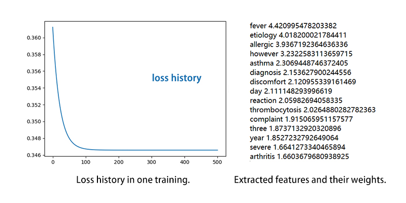
Fig. 2
As we already have the training and testing data and the labels, then we can build our system. Base on the problem we are trying to solve and the form of our input data, also according to our former experiments, we decided to use KNN as our classification algorithm. So in that case there is no training required. As our training data are some txt files each contain 15 keywords and corresponding weight, first thing is to parse the training data. We create a list to save all the symptoms and their keywords, each symptom is a dictionary and the keywords in it is the index, each keywords’ weight saved in their corresponding index. Then we writing our own KNN algorithm to compute the distance between our new input data and the training data. We use weighted L1 norm to compute the distance, which means if there is one keyword in the new input that match the keywords in our training data, then our distance minus the weight plus one, if the keyword is not in the training keywords then the distance minus the weight plus zero which equal to zero. We use a loop to compute all the keywords’ matching and after the loop is done, we output a list contain the distance of all the distance between our new input and our training data, then we use ‘argmin’ to select the smallest label as the output classifications, meanwhile we also output the second smallest and the third smallest labels as candidates.
Because each training keywords in different symptoms has different weight scale, so in order to achieve a more reasonable result, we normalize all the weights in a symptom to 1, so the result will have little influence if there is a keyword that has a much larger weight that disturb the other keywords. Even more, we averaged each distance so we won’t have a super large distance if the input sentence has a lot of keywords.
Next, after we tested our code and make sure it can achieve what we want, we use our model to test on our test dataset.
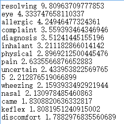
Fig. 3
According to the test result, we can achieve very high accuracy in some symptoms, like Allergy Immunology(Figure 1) and Autopsy can achieve 100% accuracy and SleepMedicine(Figure 2) and Rheumatology have 60%.
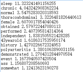
Fig. 4
But there do exist some symptoms that the accuracy is super low, like the accuracy of Surgery(Figure 3) and Neurosurgery are nearly zero.
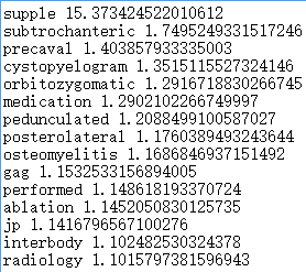
Fig. 5
We believe that this is due to the inconsistency of the training and testing dataset. The keywords we extracted from the training data is somehow a lot different from the keywords we extracted from the testing data, so when we run the test dataset on the model we trained based on training dataset, the model cannot correctly detect the similarity, then the accuracy becomes a lot lower. So the quality of the keywords we extracted from the data is really important to our system.
Final step, we tried our model on some simple sentences that we created to test the robustness of our system. See figure 6.
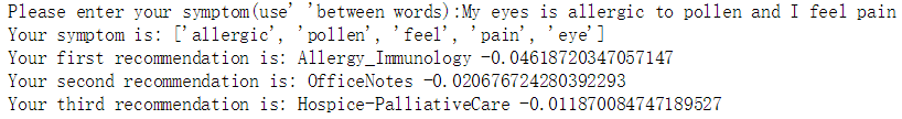
Fig. 6
The result is reasonable for some sentences, but there also have some sentences that output the less related labels. See figure 7.
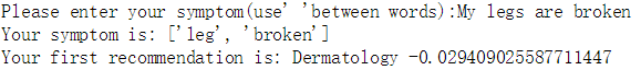
Fig. 7
We think that is due to the dataset we use is limited so the keyword we extracted from it is also limited, which mean the keywords we have may not perfectly represent the symptom we want, there exist some noisy keywords like ‘2’, ’year’ etc. So when the keywords we used to test are not that representative, the result may not that reasonable as well.
As our dataset isn’t that large and the consistency is also not so good, we would like to find a better dataset and maybe using LSTM and RNN to extract keywords is a better choice. If the system is greatly done, this system can apply to a lot of daily-life scenarios.
Jian Xu: worked on feature extraction and website design
Rongqi Ding: worked on classification algorithm design